Ed Hawkins' warming stripes make nearly two centuries of climate data instantly recognisable. But what disappears when the numbers and axes disappear too?
What if a chart lost its axis, its labels and every last number?
Normally, that sounds like a design review going rather badly but in 2018, climate scientist Ed Hawkins made it work.
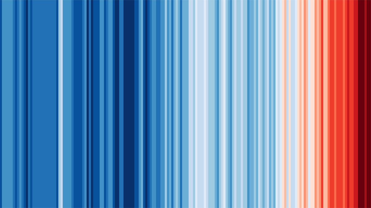
One year. One stripe.
His Warming Stripes turn annual temperatures into a row of coloured bands. Cooler-than-average years are blue; warmer-than-average years move towards red. No degree symbol to decipher. No line to follow.
Read from left to right and the colours change.
The message doesn’t need much explaining.
The stripes emerged from Hawkins’ work at the University of Reading, with an early version prepared for the 2018 Hay Festival. He was building on earlier experiments with climate-inspired knitting, rather than claiming to have invented the idea of colouring temperature data.
The original artwork, not a Coffeetableviz render. Ed Hawkins, Climate Stripes: Warming Stripes, Global 2020, digital edition 2021, University of Reading Art Collection UAC/11018. Global temperatures, 1850–2020. Reproduced intact under the artwork's Creative Commons sharing terms, with creator and collection credited.
The chart with almost nothing on it
There is a clever decision hiding inside all that simplicity, each stripe gets the same amount of room: one year. Colour carries the temperature information; the order carries time.
You don’t have to know much about charts to see the red gathering on the right. Hawkin successfully packs a lot of communication with very little furniture!
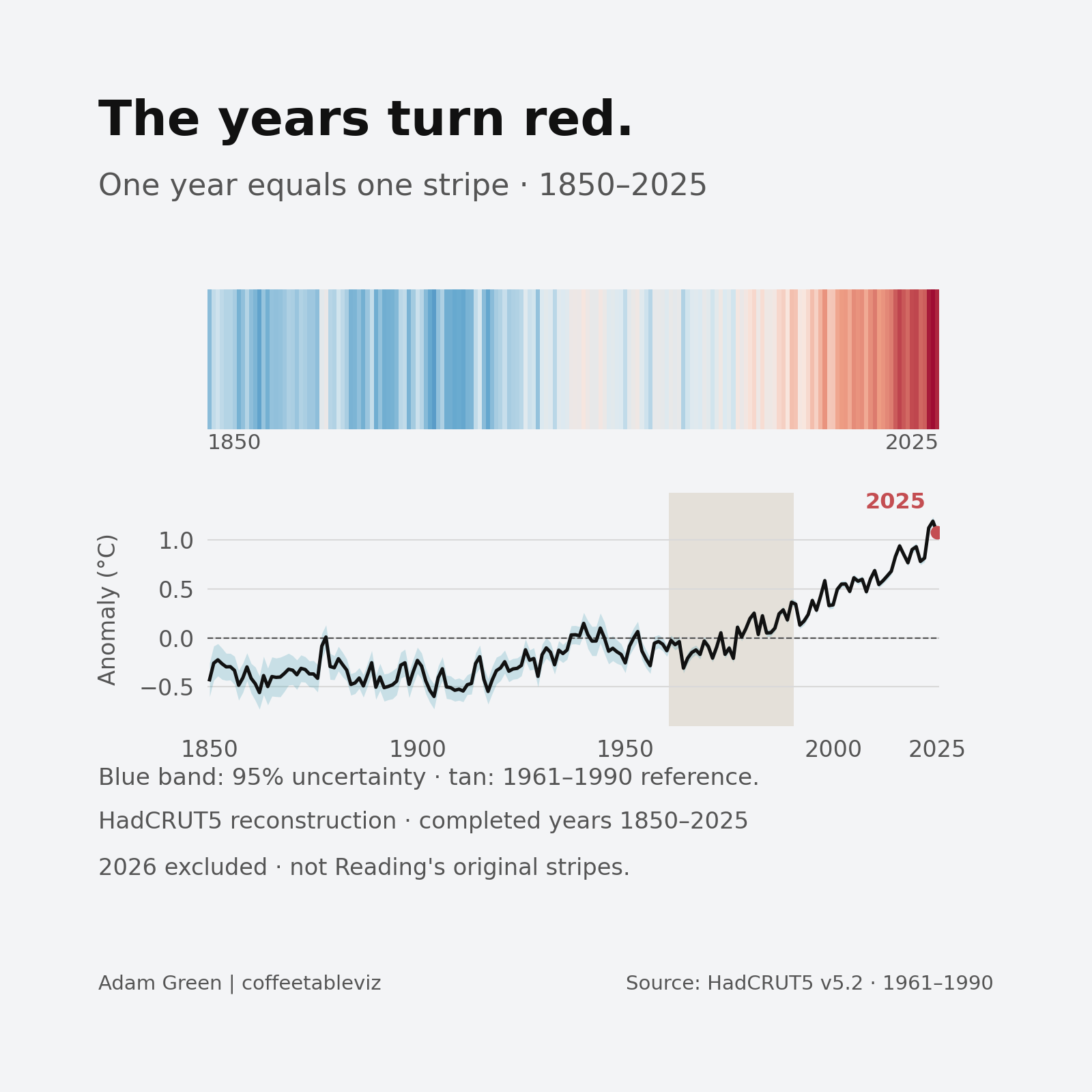
My recreation adds a little back in 🤓
The years turn red. My independent reconstruction uses the Met Office HadCRUT5 annual global analysis for 1850–2025, with the original dataset's 1961–1990 reference average. Its colours and input dataset are not pixel-for-pixel reproductions of Hawkins' historical artwork. Each stripe sits directly above the same year in the line chart. The subtle beige band highlights the 1961–1990 reference period that defines the dashed 0°C anomaly line (not an actual temperature of zero). The band also labels ≈14.0°C: a separately estimated absolute global mean for those years, reported by the Met Office Hadley Centre from Jones et al. (1999), not a value calculated from the HadCRUT5 anomaly file. Light blue shading shows the published measurement-uncertainty interval.
Why 1961? It depends which stripes.
The colours need a reference average: a period against which warmer and cooler years are judged. 1961 is not a special climate turning point. It is simply the beginning of one such averaging window.
There’s a twist. Hawkins’ earlier stripes used 1971–2000. For the 2023 update, he changed that to 1961–2010 and adjusted the colour scale to accommodate the unusually extreme temperatures while preserving the familiar look.
My Met Office reconstruction uses a different, longstanding convention: 1961–1990. None of these choices changes the actual yearly observations, but they do change which temperatures fall either side of the colour midpoint.
Beautifully clear. Deliberately incomplete.
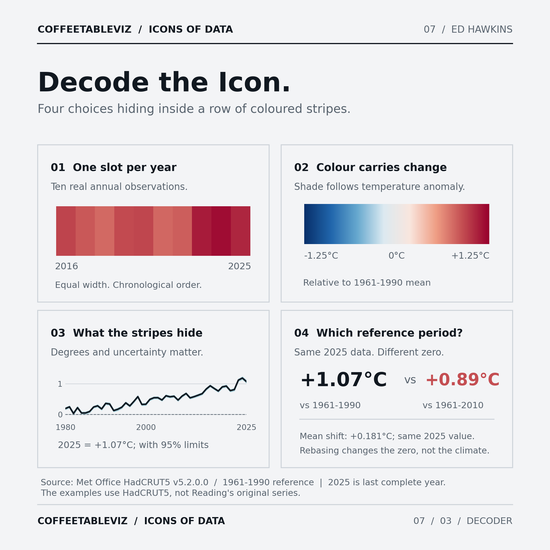
The stripes hide exact temperatures, degree labels and measurement uncertainty. Blue doesn’t mean it was cold everywhere that year; these are global annual averages, not local weather reports.
And colour alone needs a verbal explanation for people who can’t reliably distinguish the shades.
Decode the Icon: one band per year, temperature carried by colour, information restored by an axis, and the influence of the reference period. For 2025 in the same HadCRUT5 dataset: +1.07°C against 1961–1990 versus +0.89°C against 1961–2010. That isn't a change in the climate; it's a change in the chosen zero.
TLDR
Hawkins didn’t make temperature data less serious. He made the first encounter with it less demanding.
It serves as a wonderful way to start a conversation but definitely not quite the last word in it.